Menubar
All the spview tools are stored in the menubar. It contains everything needed for the spectra analysis. The menubar is composed of:
File
The File menu is dedicated to Spview project management.
Spview creates project files with the extension .spv. These files, of
xml type, contain the absolute paths of the source files used in the
project and are described in details here.
Note
Distributing .spv files from one computer to another will not allow
you to recover the project, because as mentioned above, file paths in the
xml file are absolute.
The Open Project… menu, accessible via the Ctrl + O shortcut, opens
.spvfiles.The menu Open recent is a handy menu for opening the latest projects in use. The
.spvfiles and sources must still be available and in the same place as when last used.To close the loaded project, hit Close Project or use the shortcut Ctrl + W.
The Save Project As… item (Ctrl + Shift + S) saves the project the first time, under a name to be defined. It can also be used to save the current project under another name.
The second save item, Save (Ctrl + S), saves the currently loaded project in the same location as previously defined with Save Project As….
Finally, the last element, Exit, with the shortcut (Ctrl + Q) is used to quit the application.
Data
This is the menu used to load most of the data used in the software.
The Load spectrum file menu is used to load experimental or simulated data. These can take two forms. Either a 2-column text file containing positions and intensities, or an OPUS binary file from Bruker. The file extension is irrelevant and is not taken into account. Spview first tries to define whether the loaded file is of type here. If not, it assumes that the file is of here type. Files are displayed in the central window.
The Load stick file menu handles the same files as the previous menu. However, the loaded files are displayed as stick spectra in the central window.
The Load (as stick) peak/experiment file menu loads files in the format created by the peak detector. If the file format does not meet the requirements, an error is triggered and the file is not loaded. This format, explained in details here, is the format read by the fit jobs created by XTDS. The loaded files are displayed as stick spectra in the central window.
The Load (as stick) prediction file menu is used to load files which may be in two different formats, TDS and HITRAN (2000 or 2004). As a result, Load prediction file has two sub-menus, allowing us to load one or the other. Again, the loaded files are displayed as stick spectra in the main central window.
DataManagement
This is the menu for managing data loaded into Spview. As spectra are loaded, and their data plot on screen, the file name is added to this menu.

It is then possible to Show/Hide the plots. Reload data if it has changed, and shift curves in X or Y axes with X Shift/X unshift and Y Shift/ Y unshift. Finally, you can reverse the y-axis with Y reverse.
The Restore all in basic state button, as its name suggests, resets all the states of each plot.
Assignment
Spview’s key features reside in the Assignment menu. With this menu, it is possible to load an experimental peaklist and a calculated prediction which are displayed as small ticks for each line in the top panel.
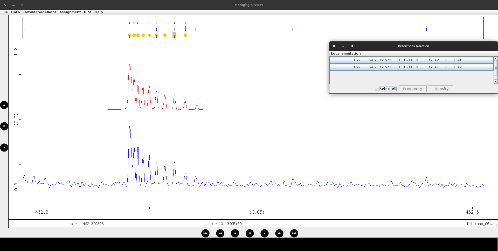
Figure above shows an example that we detail a bit below. The experimental peaklist is displayed in the upper half of this top panel. Clicking on each tick allows to select it. The lower half of the panel displays the predicted lines. Dragging a region in this part with the mouse (grayed area in the figure) deploys a popup window showing the different calculated lines lying in this region, with their quantum numbers. It is then possible to assign one or more of them (in position, intensity or both) to a previously selected experimental line. A right-click in the upper panel also allows different manipulations, like unassigning a line, changing its status (position or intensity assignment, etc). It is also possible to change the character chain that is happened to each assignment and used by the fit job created by XTDS to extract the lines to be included in the fit.
The first tool available in the menu is entitled Create a peak file from a spectrum file. It offers the possibility of detecting peaks on spectra previously loaded or not. In fact, the menu offers the option of directly opening the loaded files, or a Unknown default spectrum file name option. The algorithm used for peak detection is called “digital filter” and is explained below.

There are several options in the opened dialog.
The first is the spectrum path where the peak will be detected. It is automatically filled in if the user has chosen a spectrum already displayed. Otherwise, click on Spectrum file… to browse the files and choose the right one.
The Filter Width is the width of the single-cycle square wave as explained in the algorithm below. By default the value is of 7 and is good enough in many cases.
The Height Threshold entry defines the peak detection threshold. Enter a value higher than the noise value. It is necessary to hit Down if the peak is upside down.
X Uncertainty and Y Uncertainty are experimental uncertainties. Uncertainty Y is expressed as a percentage.
The Find Peaks button initiates peak detection, and a dialog box opens to indicate the number of peaks detected. By clicking on OK, you are encouraged to save a text file containing all the peaks. This file will be the assignment file and will be used throughout the work. You can of course click on Cancel to try another detection by changing some parameters.
The Load peak/experiment file menu loads a file in the format created by the peak detector. If the file format does not meet the requirements, an error is triggered and the file is not loaded. This format, explained in details here, is the format read by the fit jobs created by XTDS. The file name is displayed in the bottom right-hand corner of the spectrum viewer frame. Moreover, when a line is assigned, SPVIEW automatically fills this file, so there’s no need to save the assignment each time it changes.
The prediction files used in Spview can be of two different formats, TDS and HITRAN (2000 or 2004). As a result, Load prediction file has two sub-menus, allowing us to load either one or the other.
The following 2 menus, Associate experiment to data and Associate prediction to data allow you to associate experimental and simulated spectra with peak readings and predictions. The association will be effective when identical colors are assigned. The association can be removed by choosing null in the submenu.
When the assignment becomes more complex, it may be useful to save it in another file. The Save assignment file as… menu is dedicated to this. Once saved, load the new file using the Load peak/experiment file menu.
The peak finder: The Digital Filter
The method, called the “digital filter”, starts with an algorithm that convolutes the data with a single-cycle square wave of width \(W\) and amplitude 1. The data is stored as an array of integers; each data point is referenced by its offset from the beginning of the array (array index). The convolution is computed entirely by addition and subtraction, for example:
The value of the convolution for array index \(N\) is computed by summing together all of the input data points from index \(N\) to \(N+W/2\), then subtracting all of the data points from index \(N-1\) to \(N-1-W/2\). An extremum (minimum or maximum) is located where the convolution changes sign. The direction of the sign change indicates whether the extremum is a minimum or a maximum. At locations where the convolution changes sign, an interpolation is performed to locate the extremum to within a fraction of one data point spacing. The meaningful accuracy of this interpolation is a function of noise in the data and the shape of the data in the region of extremum. Figure below illustrates the operation of a digital filter.

Principle of Operation of a Digital Filter
Plot
During line assignments, it may be useful to check obs.-calc. to see if there are any outliers. To this end, this menu has two main entries: X Obs.-Calc. and Y Obs.-Calc. respectively used for position and intensity fits.
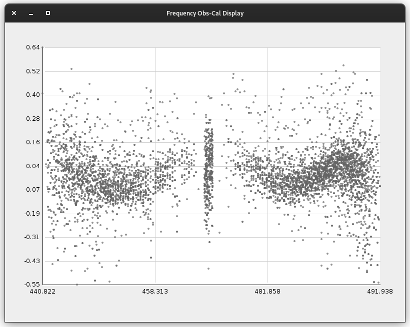
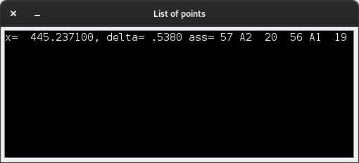
A single-click on a data point, as shown in the figure below, opens a new window providing the information needed to identify the line. In addition, a double-click the on the point, and the main window zooms in and moves to the relevant region of the spectrum, placing the possible outlier in the center.
Help
This menu opens the About window, detailing the software and copyrights. Click here to see the text of this dialog box.